For the final project in our Deep Learning class, we used a convolutional autoencoder to restore damaged images. Arriving at the final model architecture was harder than it might seem, so in this article I’ll explain the project and learnings we had.

An autoencoder is characterized by its two halves that are usually symmetrical: the encoder and the decoder. First, the encoder transforms the input into a compressed representation containing all important information about the input. This is then fed to the decoder, which transforms the compressed input back to the original size. In the process, finer information like noise is discarded, while the important parts are kept. This makes it a good starting point for restoring damaged images!

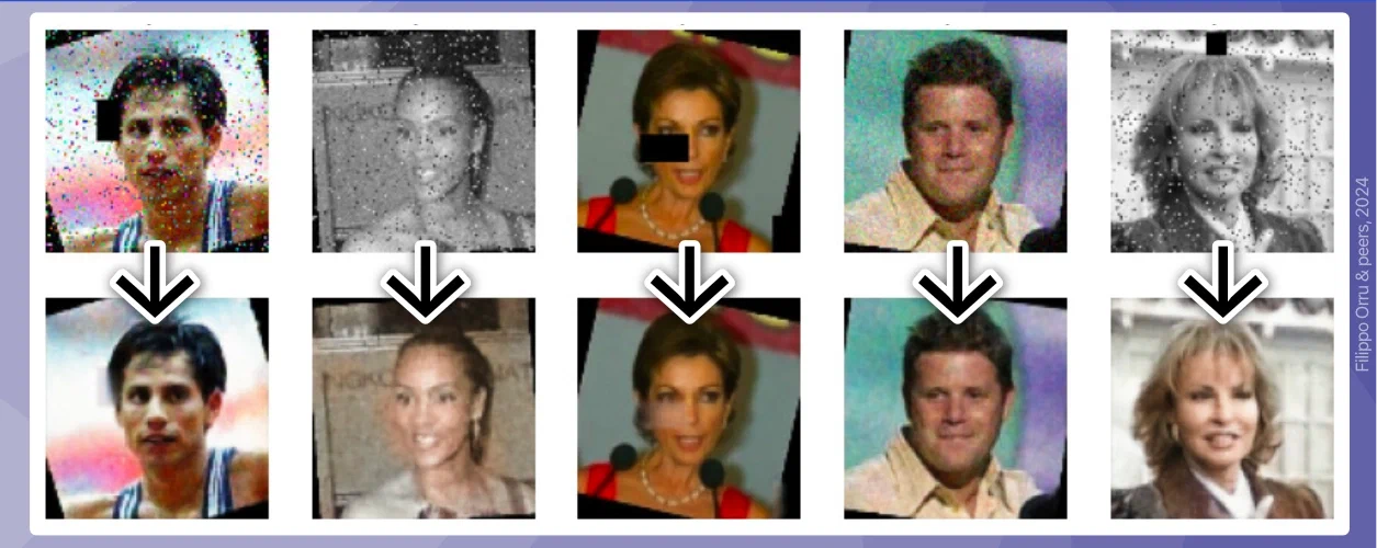
We applied these types of “damage” to the input data:

1. Additive gaussian noise
2. Flipping some pixels to random values
3. Occlude parts of the image with square patches
4. Desaturate to grayscale

# Dataset

The dataset we used, Labeled Faces in the Wild (LFW), contains more than 13,000 face photographs of over a thousand individuals, collected from the web. Every person has two or more distinct photos in the data set. The dataset contains two versions of each image, namely the original and a funneled version. In this context, funneling means aligning a face so that the eyes and mouth are at fixed positions within the image frame. This reduces variation between different images, which allows the neural network to focus on learning about facial features in a controlled manner. This improves performance and training efficiency.

# Finding a Good Model

Initially, we started with a simple setup based on Tensorflow’s autoencoder tutorial. It consists of a few convolutional layers, each downsampling the input’s dimensions, then followed by transposed convolutional layers, which perform the reverse operation. However, in our initial model, we used simple MaxPooling and Upsampling operations to reduce the dimensions. This model performed quite poorly. It was able to take intact images as input, compress them, and reconstruct the input, but unable to correct noisy images with sufficient detail.

We were inspired by the papers Image Restoration Using Convolutional Auto-encoders with Symmetric Skip Connections (Mao, 2016), and U-Net: Convolutional Networks for Biomedical Image Segmentation (Ronneberger, 2015). Based on this research, we implemented two key improvements:

1. We switched from our MaxPooling and Upsampling layers to using convolutions and transposed convolutions with a stride of (2, 2), which allows the model to learn which pixels are relevant when downsampling and upsampling.
2. We introduced skip connections to our model, shown in the next image. This means that the output of each encoder layer is fed to its corresponding decoder layer, enabling later decoder layers to restore fine details that were lost when compressing the input in previous layers.

The model is made up of multiple encoder blocks that compress the image, then the same number of decoder blocks. The output dimensions are the same as the input dimensions.

The encoder block is very simple. It just performs two convolutions, one of which downsamples the input to half of its x and y dimensions. Afterward, we apply dropout and batch normalization to improve the model’s generalization.

In the decoder, we want to concatenate the input with the corresponding encoder’s output (or the actual input image, in the case of the last decoder). To do this, we first upsample the image with a transposed convolution, concatenate it with the skip connection input, and apply two more convolutions.

# Conclusion

This worked much better than expected! We trained a convolutional autoencoder with some advanced features. It is able to correct quite intense levels of grain, pixel flips, and to some extent even desaturation.

Plotting the training and validation loss reveals no signs of overfitting, so maybe we could have improved the model’s performance even more with more training. I also feel like a larger number of kernels and a size of 5x5 would be worth exploring. For our final project report, we conducted a hyperparameter search, comparing 7 variations of the base model using different kernel sizes, numbers of layers, and with or without skip connections. The following image shows the input image, the results of training these variations for 20 epochs, and the ground truth image.

However, the model has some limitations. First, while images sized 48x48 pixels were fine, performance suffered greatly when we tried using images of 128x128 pixels. This is likely because the model’s architecture is static – we always apply the same convolutional kernels with size 3x3, no matter the image size. On a larger image, this results in a relatively smaller receptive field.

We also tried rotating the images randomly, but the model was not able to restore the original orientation. The same applies to randomly flipping the image vertically.

Lastly, I want to say that working on this project with my three colleagues was a pretty good learning experience. What I enjoyed most was the process of reading a paper, implementing some changes to the model, and seeing the improvements.

# More

• Read how I redesigned this site.
• Want to hear about another project? How I built a split keyboard.
• Or you can read about me.

All figures in this post were drawn by me.